Introduction

Identifying people based on their audio is a fascinating topic. Every human voice is distinctive; as people age, their voices vary, and they sound different in different contexts, altering the problem landscape correspondingly. Speaker Identification is concerned with identifying a person based on the spoken audio of that person. Traditionally, speech processing models were widely recognized, but convolution neural networks have lately demonstrated that they, too, may generate astounding outcomes.

Data Description

I was always interested to train a model in my language. Therefore, I collected Nepali audio from youtube of exactly 34 politicians male and female speaking at different venues, providing proper care not to include noise in the audio and the average audio length is around 5 minutes. The dataset is available here

Converting to Deep Learning Problem

Showing the formulation of deep learning problem

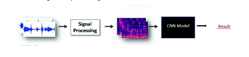
The necessary preprocessing is done depending upon the audio we have it may include removing some part of the audio, removing silence, etc. As CNN can only work on images (1d CNN can word on text but not considering here), the spectrogram images is created from the preprocessed audio and provided as input to the model which will perform training to produce the result. Basically there are four steps:

Reading the audio
Perform necessary pre-processsing
Selecting a Model
Preparing data for the model
Model Architecture

1. Reading the audio

The first step in this many step process is reading an audio, the audio can be in many format .wav, .mp3, etc. It can be done my using signal processing library Librosa.

Reading the audio

import librosa
path= ‘path to audio’sample_rate= 22050
arr_audio,_=librosa.load(path,sr= sample_rate) #arr_audio is an array of amplitudes if the audio is 2sec in length
#it will be (2,2*22050)= (2,44100), where 2 in the array is due to #dual channel of audio

As audio is nothing more than a signal, where on the x-axis there is time and on the y-axis, there is amplitude, as it is a continuous signal we want to convert in a discrete form so that we can extract the features from it. By sampling the signal at a specific rate we can do this, what does it mean is that we are getting the value of amplitude from some instances of time. Here the sampling rate is 22050, meaning on one second of audio we will extract the amplitude 22050.

2. Preprocessing

2.1 Converting to mono channel

As the audio data is from youtube, it is a dual-channel meaning for the particular instance of time, there is two value of amplitude one for the left earpiece and one for the right. But we need a single value of amplitude at any instance. So just by taking the mean of the dual-channel amplitude array, we can convert it into a mono channel.

arr_audio= arr_audio.sum(0)/2

2.2 Removing noise

In every audio, the first 1 minute is an advertisement or some other kind of unwanted audio segment. So we will be removing the first and the last 1 minute from every audio.

arr_audio= arr_audio[sample_rate60:arr_audio.shape[0]-sample_rate60]

2.3 Removing silence

While speaking they may we momentary pause in between, we want our model to learn the characteristics of individual persons audio, it will learn nothing from the silence. So the silence needs to be removed.

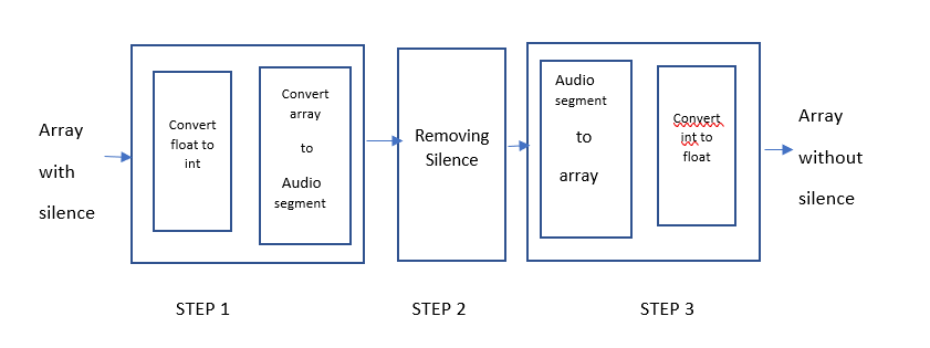
Steps to remove silence

from pydub import AudioSegment
from pydub.silence import split_on_silencedef float_to_int(array, type=np.int16):
if array.dtype == type:
return array if array.dtype not in [np.int16, np.int32, np.int64]:
if np.max(np.abs(array)) == 0:
array[:] = 0
array = type(array * np.iinfo(type).max)
else:
array = type(array / np.max(np.abs(array)) * np.iinfo(type).max)
return arraydef int_to_float(array, type=np.float32):
if array.dtype == type:
return array if array.dtype not in [np.float16, np.float32, np.float64]:
if np.max(np.abs(array)) == 0:
array = array.astype(np.float32)
array[:] = 0
else:
array = array.astype(np.float32) / np.max(np.abs(array))
return array#Step1:Create an convert to int and create audio_segment#Convert to float
feature= float_to_int(arr_audio)#Create audio segment
audio = AudioSegment(feature.tobytes(),frame_rate = self.sample_rate,sample_width = feature.dtype.itemsize\
,channels = 1) #Step2:removing the silence from the audio segment
audio_chunks= split_on_silence(audio,min_silence_len=min_silence,silence_thresh= -30,keep_silence= 100)
#Step3:converting it back to the array
#Convert audio segment to array
arr_audio= sum(audio_chunks)
arr_audio= np.array(arr_audio.get_array_of_samples())#Convert back to int
arr_audio= self.int_to_float(arr_audio)

After doing all the preprocessing the data looks like this:

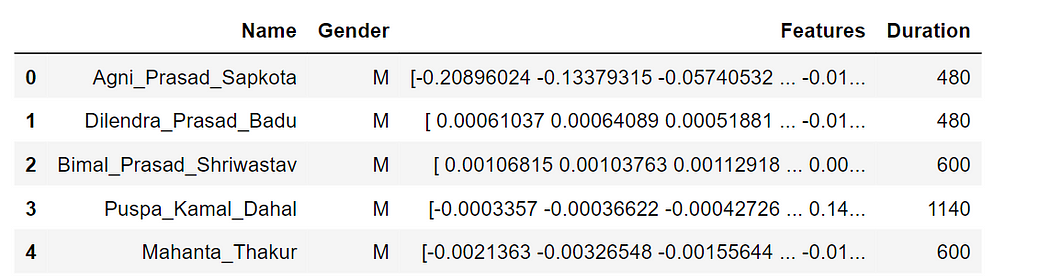
A single data point contains the name of the speaker, its gender, Duration meaning the length of the audio in seconds, and finally Features that contain the amplitude of the audio sampled at a specific sampling rate.

3. Selecting a model

There are 34 speakers if we consider each speaker as a single class there will be 34 classes. As the speaker increases, the class will also increase which is not an ideal scenario. To identify a single class supposes k1, the model needs to learn features that clearly distinguish it from other (K-k1) classes which will require lots of data ie increasing the length of audio of a single speaker. I don’t think a user wants to spend time recording its audio, he/she is willing to record for 5–30 sec and get done with it. So, using this strategy is not a choice.

A Siamese Network is a network that contains two identical subnetworks ‘identical’ here means, they have the same configuration with the same parameters and weights. Parameter updating is mirrored across both sub-networks. It is used to find the similarity of the inputs by comparing their feature vectors, so these networks are used in many applications.

If we want to add a new speaker here we can update the neural network and retrain it on the whole dataset which was not possible in traditional architecture. SNNs, on the other hand, learn a similarity function. Thus, we can train it to see if the two images are the same (which we will do here). This enables us to classify new speakers without training the network again.

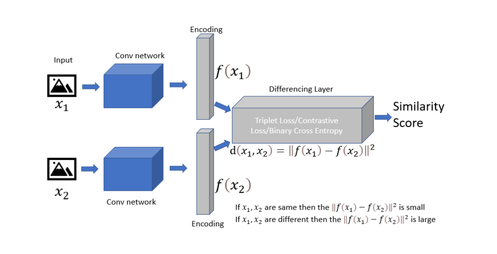
Siamese Network.(https://medium.com/swlh/one-shot-learning-with-siamese-network-1c7404c35fda)

Siamese networks accept two inputs x1 and x2. For our case, it is either two spectrogram images from the same user or from different users. Images from the same user are labeled as 1 and images from different users are labeled as 0. These images are sent through an identical network and feature vectors f(x1) and f(x2) are generated. A function is used to calculate the difference between these two feature vectors. The difference score between the feature vector for the same user will be small as they will be located in the same neighborhood in that dimensional space whereas for the different users the feature vector difference will be large.

Lets take example the two feature vector are (0.5,0.7) and (1,0.7)

Different User:

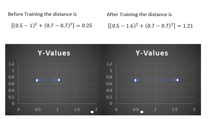
As we can see the model tries to increase the distance between the feature vector if they are from different user.

From same user:

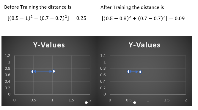
Similarly if the feature vectors is from same user after every iteration model reduces the distance between the two bringing them closer in the vector space.

4. Preparing data for siamese network

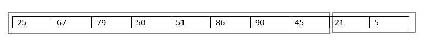
Let’s suppose there is an audio from speaker Hari of 0.3miliSeconds and by using the sampling rate= 22050, we can compute amplitude at 8 instances ie (0.3*1000 sec)/22050~10. SO, the feature vector for this audio segment looks like this:

1. Train test splitting

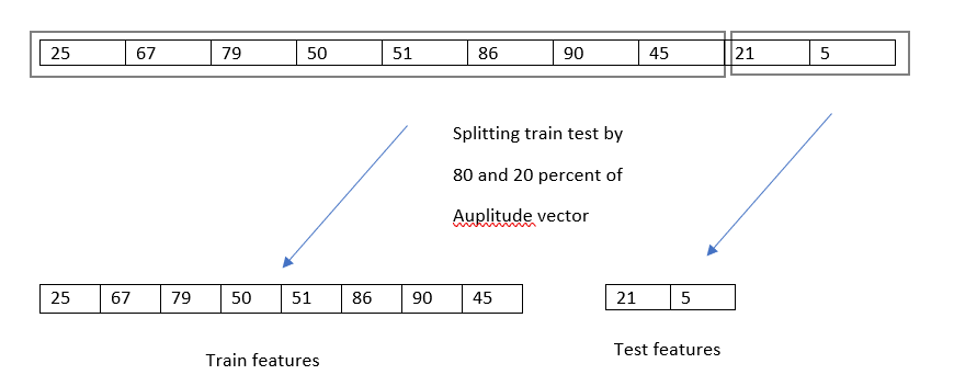
The first 80% of the audio segment was utilized to generate a training set, while the remaining 20% was used to create the test set.

2 Getting similar and disimilar pairs of spectogram from speakers audio

2.1 Similar pair:

A single pair of the image of spectrogram created from the specific user audio will create one data point and the label of this data point will be 1 indicating that this pair of spectrogram images belong to individual audio.

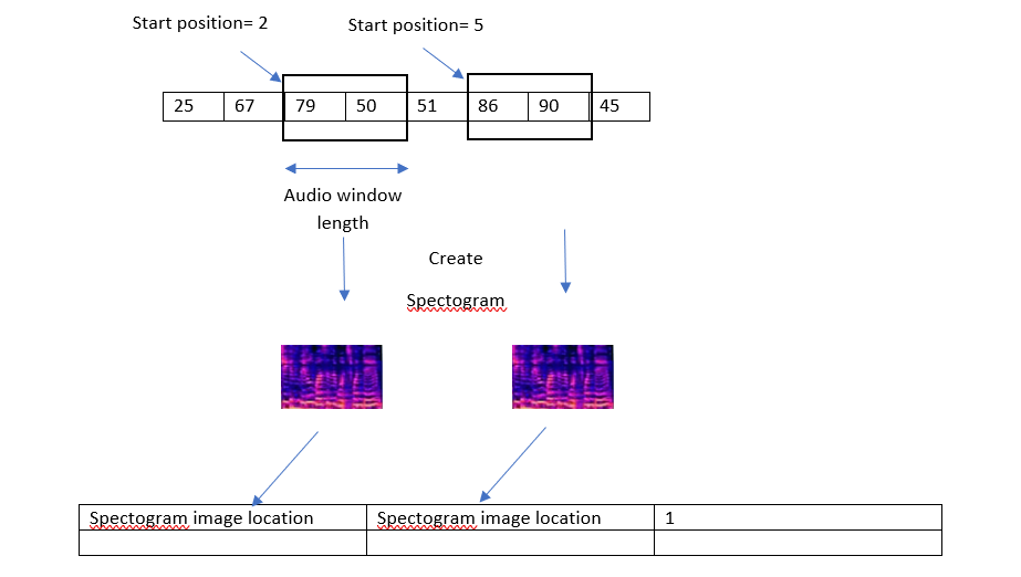
The most important parameter while creating a spectrogram is the audio window length which defines the length of the audio segment which will be used to create a single spectrogram image. Similarly, the starting position for these two windows will be selected randomly. For my implementation, I have selected 100 pairs of datapoint for an single user, therefore the total datapoint which will have label 1 are 34*100= 3400.

2.2 Dissimilar pair:

A single data point contains one spectrogram from one user and another spectrogram from another user, with the label 0 indicating that the spectrograms belongs to a separate user. As a result, we will pair each user with every other user and construct all possible combinations of pairs from distinct users.

We chose 25 pairs of spectrogram photographs, one from each of two different people. As a result, we will generate 25 pairs of spectrograms with each other user for each user (33 in our situation), for a total of 3325= 825 pairs of images. Similarly, the total number of dissimilar spectrogram pairings for 34 persons is 34825=28050, and these pairs are labeled as 0, indicating that the spectrogram images in the pair are from distinct people.

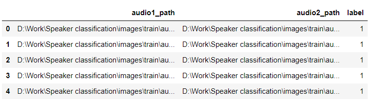
The dataset looks like this after performing all these tasks:

4 Model Architecture

Because the image number is just 31000, transfer learning is the only option. As a result, DenseNet121, which has already been trained on “imagenet,” is employed here. We must utilize the spectrogram height and breadth that we created while initializing this network.

subnetwork= tf.keras.applications.densenet.DenseNet121(include_top=False, weights=’imagenet’, ,input_tensor=None,input_shape=(height,width,3), pooling=None)

Similarly, we need a distance function which calculates the distance between two feature vector produced by the DenseNet. For this purpose we will be using euclidean distance:

def euclidean_distance(self,inp): x,y= inp
sum_square = tf.math.reduce_sum(tf.math.square(x - y),axis=1,keepdims=True)
return tf.math.sqrt(tf.math.maximum(sum_square,1e-07))

Finally, let’s put all the pieces together and create a complete model.

def create_siamese_network(height,width):
#Inputs for two spectrogram images
image1= Input(shape=(height,width,3))
image2= Input(shape=(height,width,3)) #sending the images through the DenseNet
output1= Flatten()(subnetwork(image1))
output2= Flatten()(subnetwork(image2)) #Calculating the distance between the feature vector
output = layers.Lambda(euclidean_distance)([output1, output2])

    model= Model(inputs=[image1,image2],outputs=output)  
    return model

DenseNet will generate a feature matrix with multiple channels; to get a vector from it, we flatten the output matrix and calculate the distance between the channels.

5. Training the model

5.1 Contractive Loss

We need a loss function that minimizes the distance between spectrograms from the same individual and maximizes the distance between spectrograms of a different individual. Contractive loss works exactly like that and we will be using it here to train the model.

margin= 3.0
def contractive_loss(label,distance):

difference= margin-distance  
temp= tf.where(tf.less(difference,[0.0]),[0.0],difference)     
loss= tf.math.reduce_mean(tf.cast(label,dtype=tf.float32)*tf.math.square(distance)+(1-tf.cast(label,dtype=tf.float32))*tf.math.square(temp))  
  
return loss

The margin value is the most crucial parameter in the contractive loss. This number tells the model what the minimal distance between feature vectors from different persons should be, and we set the margin value to 3 in our implementation. Similarly, the model attempts to reduce the distance between spectrograms of the same image to 0.

5.2 Evaluation

similar distance= The distance between the feature vectors of two spectrogram images generated from the same person.

dissimilar distance= The distance between the feature vectors of two spectrogram images generated from the different person.

At first, the similar and dissimilar distances were almost identical, but as the model trained, they began to diverge, and after 30 epochs, the distance between training and testing looks like this:

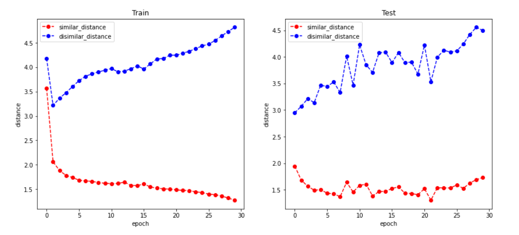
Epoch vs Distance

For the training set, the average distance between spectrograms of the same individual was 1.4, whereas the distance between spectrograms of different people was 4.7. Similarly, the average similar distance was 1.8 and the average dissimilar distance was 4.4 for the test set.

Because the model simply outputs the value of the distance between the pairings, we can conclude that if the distance between the pairs is less than 1.8, we will label it as 1, and else it will be labeled as 0.

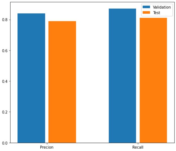
The precision and recall values for the training set were determined to be 0.87 and 0.84, respectively, whereas the precision and recall values for the test set were close to 0.8.

6. Training Parameter

The model was trained for 30 epochs with a learning rate of 1e-4. The Adam optimizer was employed, with a polynomial learning rate decay and the first 100 steps of the models operating as warn steps.